In a nutshell

We know analytical calculus (aka handwritten math). But as we know, it becomes difficult once we step out of the classroom into the real world. So we wanna use complex equations with many constraints to find important values. But we do not wanna do it by hand.

What to use then? Numerical Calculus. Basically we use numbers along with certain algorithms to find the values we want.

Why not solve by hand?

For example, let’s say we have a system of 3 equations for variables \(x, y, z\). But there’s a catch: x, y, z show up in derivative forms.

\[\begin{aligned} \frac{dx}{dt} &= \sigma (y - x), \\ \frac{dy}{dt} &= x (\rho - z) - y, \\ \frac{dz}{dt} &= xy - \beta z, \end{aligned}\]

Where \(\sigma, \rho, \beta\) are some arbitrary constants
And initial conditions \(x(0) = 1,\quad y(0) = 1,\quad z(0) = 1.\)

If you’re curious, the above is a simple example of the Lorenz System¹

Honestly, we do not wanna solve it by hand (unless you enjoy the math pain). So we can try to guess what \(x, y, z\) could be. But we would need very educated guesses if we wanna get to a solution someday.

Or, we can use a clever algorithm like Runge-Kutta² where we plug our equations into some functions and calculate numbers to get approximated solutions.

Is it actually better than handmade solutions?

It depends. For small stuff, you can do it by hand. For complex scenarios, you could try using WolframAlpha or MATLAB Symbolic ToolBox. But when it gets tough, numerical methods are pretty handy and commonly applied.

It is a good alternative because computers are good with numbers. So we can give our weird-looking algorithm to the computer via code, compile it, and have it loop through the equation a couple hundred times (which it does very very quickly). And boom, we have the magical numbers.

Note, numerical methods usually mean some sacrifice in precision. Also, you may not get a general solution, since numerical methods work with numbers; our computers deal with numbers.

In short: You need numbers, your computer will deal with numbers, and you need a good algorithm to compute those numbers.

Numerical methods can be used in many cases: looking for roots, regression, integrals and derivatives, differential equations, etc… pretty much any calculation that can be done with specific numbers.

Tools like MATLAB already have plenty of these techniques implemented, like the \ operator or the ode45 function. But as a way of self-practice, we’ll go through a few methods worth mentioning and code it ourselves.

Note: I won’t go into the details. If you are really into numerical methods, I recommend this book.

Error and precision

Using numerical methods usually implies some sacrifice in precision. However, we should be clear about how much we’re willing to give in, considering more precision = more iterations. Something we can do is have the program calculate how much the values are changing in each iteration, and have it stop when a new value changes less than 5%, or any number you’d like.

Let’s define the approximate error like this:

\[e_{i+1} = \left| \frac{x_{i+1}-x_i}{x_{i+1}} \right|\]

Where \(x_n\) is the values calculated by our method.
Multiply the above equation by 100 if you like percentages.

I’ll be using the above for the methods developed below.

Roots of Equations

Adapted from pg 117³

Let’s say we want to know the root of a function like \(x^2 + x + 1\). Easy enough: quadratic formula, right?
But let’s step it up: \(f(x) = e^{-x}-x\). Of course, not all cases would behave weirdly, but it is likely we wanna know the values of x for which \(f(x) = 0\). Since this deals with numbers, it is a good way to start with numerical methods on code. So let’s make some code that calculates that.

Bracketing Methods

Adapted from pg 123³

Imagine we have \(f(x) = e^{-x}-x\). And we wanna know when \(f(x)=0\). You can try it by hand (spoiler alert: it’s hard, you won’t get a solution).

Or, a simple simple way to know is to simply print its graph.

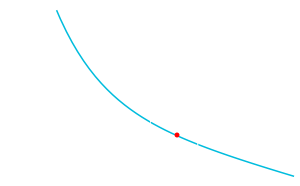
Taken from WolframAlpha

With the graph, we can see the root is around \(x=0.5\). Close enough, but we’d like to have a closer approximation.

Something we can do is use some theory to help us make an algorithm:

Intermediate Value Theorem: If a continuous function \(f(x)\) takes on values \(f(x_1), f(x_2)\) at two points \(x_1, x_2\), and if \(f(x_1)\) and \(f(x_2)\) have opposite signs, then there must be at least one root between \(x_1\) and \(x_2\).

In English, we can pick two numbers \(x_1, x_2\) and see the sign of \(f(x)\). If \(f(x_1)\) and \(f(x_2)\) have different sign (one is positive and one is negative), we know for sure there is a root somewhere between \(x_1\) and \(x_2\).

For example, in the graph we see that \(f(0)\) is positive, and \(f(1)\) is negative. And we know it is continuous (does not jump randomly between 0 and 1). Therefore, we know there is at least one root between 0 and 1.

From here, bracketing methods are born: we have a bracket, a range of possible numbers \(x_1, x_2\), where we know there is at least 1 root.

1. Bisection

Adapted from pg 127³

The brute-force approach:

1. Guess an upper and lower bound, \(x_{upper}, x_{lower}\)
2. Calculate \(f(x_{upper}), f(x_{lower})\)
3. If \(f(x_{upper}) \times f(x_{lower}) < 0\), there is at least 1 root between \(x_{upper}, x_{lower}\)
4. Use the bisection equation:

\[x_{guess} = \frac{x_{upper} + x_{lower}}{2}\]

Let \(m = f(x_{guess}) \times f(x_{lower})\)

• If \(m<0\), the root is in the interval \([x_{lower}, x_{guess}]\).
  Set \(x_{upper} = x_{guess}\) and go back to step 4.
• If \(m>0\), the root is in the interval \([x_{guess}, x_{upper}]\).
  Set \(x_{lower} = x_{guess}\) and go back to step 4.
• If \(m=0\), the root is in \(x_{guess}\). We have our solution.

2. False-Position

pg 135

Open Methods

pg 145

1. Newton-Raphson

pg 151

2. Secant

pg 157

3. Brent’s Method

pg 162

4. Multiple Roots

pg 166

Polynomials

pg 176

1. Muller’s Method

pg 183

2. Bairstow’s Method

pg 187

Examples

Linear Equations

pg 231

Gauss

pg 245

rref

pg 273

Gauss-Seidel

pg 304

Examples

Optimization

pg 345

??

Regression

pg 456

Least Squares

pg 456

Linear

pg 456

Polynomial

pg 472

General

pg 479

Interpolation

pg 490

Newton

pg 491

Lagrange

pg 502

Fourier

pg 526

Numerical Calculus

pg 587

Trapezoidal

pg 605

Simpson

pg 615

Unequal segments

pg 624

Integration

pg 633

Romberg

pg 634

Adaptive

pg 640

Gauss

pg 642

Improper integrals

pg 650

Partial Derivatives

pg 662

ODEs

pg 699

Runge Kutta

pg 709

Stiffness, multistep

pg 755

Boundary value

pg 781

Eigenvalues

pg 789

PDEs

pg 845

Laplace

pg 852

Crank-Nicolson

pg 882

Finite-Element

pg 890

nmat

• fix functions
• optimize functions
• comments
• equations docs
• documentation

Credits